By Jacob Harris
Cornell University, Roper Center for Public Opinion
ASCII (short for American Standard Code For Information Interchange) is a standard format for storing data that requires minimal storage space and can be handled by almost all computers and programs. There are a huge number of datasets stored only in ASCII format and thus not easily accessible to many researchers. These need only be converted from ASCII files to modern data formats to be ready for analysis. This document explains how ASCII files can be converted in R and presents custom functions that remove much of the tedium involved with ASCII conversions and reduce the likelihood of data errors.
ASCII documentation basics
When converting an ASCII file, you need the data file itself and a separate page that documents the variables in the ASCII dataset. Here is an example of a documentation page:
Figure 1.
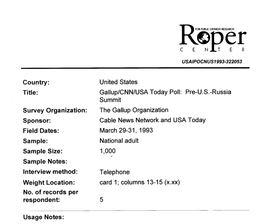
The most important information on this page for our purposes are the “Weight Location” and the “No. of records per respondent.” From here on, records are referred to as “cards,” meaning there are five “cards” accompanying this ASCII file. I will give more detail on the “Weight Location” input later.
Setting up your R script
Your R script will be broken down into several different sections. Sections 2-4 will repeat for each card in the dataset. It will look something like this:
#### Set up ####
#### Card 1 ####
#### Card 1 question labels ####
#### Card 1 value labels ####
#### Card 2 ####
#### Card 2 question labels ####
#### Card 2 value labels ####
#### Merge cards ####
#### Save out data ####
In the “Set up” section of your script you will need to include the following code:
#### Set up ####
remove(list = ls())
library(speedycode)
library(readroper)
library(dplyr)
library(sjlabelled)
library(labelled)
library(haven)
library(devtools)
library(stringr)
library(purrr)
Reading ASCII files using the read_rpr function
Below is the code for reading an ASCII file and converting it to a modern format. Use this link to view the full documentation and download the ASCII file so you can follow along. The link also contains a template for converting ASCII files in R you can use in the future.
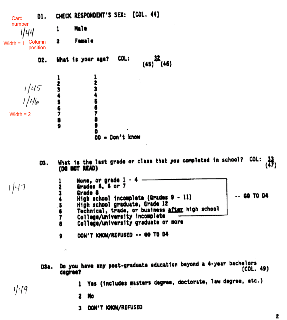
As the data name indicates, the code below reads in the first card out of five for this dataset. Cards must be read in separately and then merged later. In the documentation, each question has two numbers split by a backslash. The first number indicates the card number, meaning that all of these variables come from card 1. The second number indicates the column position for that card number. Each column can only contain one character (almost always a number) so some questions will require more than one column. For instance, age variables typically use two columns since it requires two numbers to record that someone is 30 years old. The number of columns used to record a variable is also known as the width. Card number, column position, and width are all you need to convert an ASCII file!
See below how the code aligns with the ASCII documentation in Figure 2. For the first question, the card number is one, the column position is 44, and the width is 1 (this is just a sample of the documentation so this page starts at column 44). If you refer to Figure 1, you will see the information needed to convert the weight variable. It begins on column 13, it has a width of 3 because it ends on column 15, and it is a part of card 1.
Figure 2
card1 <- read_rpr(
col_positions = c(13,29,30,44,45,47,48,49,53,78,80),
widths = c(3,1,1,1,2,1,1,1,2,2,1),
col_names = c("Weight", "Region", 'Stratum', "Sex", "Age", "Education", "Race",
"PostGradEducation", "Income", "State", "AgeSummary"),
filepath = "YOUR-file-path-here",
card_read = 1,
cards = 5
)
And look at that, we have a nice-looking dataset! (only the first 10 observations are shown). At this point, the ASCII file has already been converted. Everything from this point on deals with a few necessary but minor adjustments, labeling the data, checking the data for errors, and outlining some custom functions to make the conversion process more efficient :
head(card1, n = 10)
## # A tibble: 10 × 11
## Weight Region Stratum Sex Age Education Race PostGradEducation Income
## <chr> <dbl> <dbl> <dbl> <chr> <dbl> <dbl> <dbl> <chr>
## 1 056 3 3 2 54 7 2 NA 03
## 2 062 3 3 1 23 7 1 NA 04
## 3 271 2 3 1 31 4 1 NA 06
## 4 087 3 3 2 49 7 1 NA 05
## 5 113 3 2 2 42 7 1 NA 03
## 6 059 2 3 1 38 8 1 2 05
## 7 064 3 2 2 70 8 1 1 04
## 8 092 3 3 2 67 5 1 NA 08
## 9 170 1 3 2 78 3 1 NA 01
## 10 178 3 1 2 00 3 1 NA 02
## # … with 2 more variables: State <dbl>, AgeSummary <dbl>
Including weight variables
When accounting for weights in ASCII conversions, there are two things you need to do. First, you must find where the weight variable is. Weights don’t show up in the normal flow of survey questions. Instead, they are usually placed near the beginning of the documentation. See Figure 1 and you will see that the weight variable for this dataset is in card 1, in columns 13 through 15, and has a width of three (because it takes up three columns). That is all you need to know! Refer back to the code above and you will see how the weight variable is accounted for. Of course, weights are only relevant in some survey data files so if you are not working with survey you do not need to worry about this.
The second issue with weight variables is making sure the decimal points are where they should be. ASCII files almost never have decimal points in the right place so you need to do this on your own. The code below converts the weight variable to numeric and then divides it by 100 to align the decimal points. I know to divide it by 100 because the information given about the weight variable on the first page of the documentation has “x.xx” which means that the decimal needs to move to the left two places. If you aren’t sure if the decimal is in the right spot or the documentation isn’t clear, take the mean of the weight and it should be almost exactly equal to 1. If the mean is 10 or 0.1, for instance, you need to adjust the decimal placement.
card1 <- card1 %>%
mutate(Weight = as.numeric(Weight),
Weight = Weight/100)
Labelling the data
Now that the data has been successfully converted, the next step is to provide clear and accurate labels. Coding all the variable and value labels, however, can become quite cumbersome. To speed this up, there are a few custom functions you can use. These will be described in detail at the end of the tutorial. For now, here is a quick overview of how labeling works.
An initial step before labeling the variables is converting them all to the numeric variable class. The labeled package, which is what I use for labeling, will return an error if you try to label a non-numeric variable.[1] Typically, all the variable values should be numbers in the first place, but that still doesn’t mean they are all stored as numeric variables in R (use the class and str commands to quickly view the classes of each variable). Use the following code to convert all variables to numeric:
card1 <- card1 %>%
mutate_all(as.numeric)
If this returns an error, there are probably some non-numeric characters in your data. Fortunately, this is rare. If it does occur, however, you will need to convert the character values to numbers. It doesn’t matter what numbers you choose as long as you keep track of the substantive information they are linked to. Your code for doing so may look something like this (The number you use is completely up to you. I use 99 so it doesn’t get confused with other values in the variable):
card1 <- card1 %>%
mutate(Q1 = case_when(Q1 == "X" ~ 99,
T ~ Q1))
Now, let’s use a different page from the documentation (Figure 3) for an example of how labeling works.
Figure 3
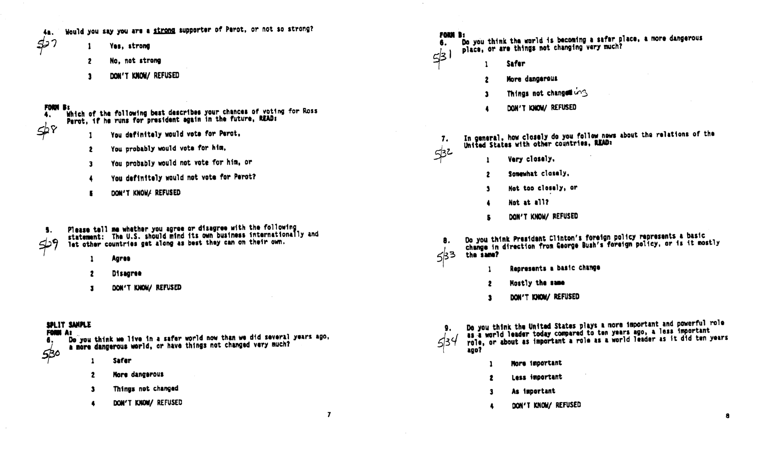 Here is the code used to create the labels for this portion of the dataset. Looking at Figure 3, you can see how the variable names and labels intuitively align with one another.
card5 <- card5 %>%
set_variable_labels(
Q4a2 = "Would you say you are a strong supporter of Perot, or not so
strong?",
Q4b = "Which of the following best describes your chances of voting
for Ross Perot, if he runs for president again in the future?",
Q5 = "Please tell me whether you agree or disagree with the
following statement: The U.S. should mind its own business
internationally and let other countries get along as best they can
on their own.",
Q6a = "Do you think we live in a safer world now than we did several
years ago, a more dangerous world, or have things not changed very
much?",
Q6b = "Do you think the world is becoming a safer place, a more
dangerous place, or are things not changing very much?",
Q7 = "In general, how closely do you follow news about the relations
of the United States with other countries?",
Q8 = "Do you think President Clinton's foreign policy represents a
basic change in direction from George Bush's foreign policy, or is
it mostly the same?",
Q9 = "Do you think the United States plays a more important and
powerful role as a world leader today compared to ten years ago, a
less important role, or about as important a role as a world leader
as it did ten years ago?") %>%
set_value_labels(Q4a2 = c(
"Yes, strong" = 1,
"No, not strong" = 2,
"DK/Refused" = 3),
Q4b = c(
"You definitely would vote for Perot" = 1,
"You probably would vote for him" = 2,
"You probably would not vote for him" = 3,
"You definitely would not vote for Perot" = 4,
"DK/refused" = 5),
Q5 = c(
"Agree" = 1,
"Disagree" = 2,
"DK/Refused" = 3),
Q6a = c(
"Safer" = 1,
"More dangerous" = 2,
"Things not changed" = 3,
"DK/Refused" = 4),
Q6b = c(
"Safer" = 1,
"More dangerous" = 2,
"Things not changed" = 3,
"DK/Refused" = 4),
Q7 = c(
"Very closely" = 1,
"Somewhat closely" = 2,
"Not too closely" = 3,
"Not at all" = 4,
"DK/Refused" = 5),
Q8 = c(
"Represents a basic change" = 1,
"Mostly the same" = 2,
"DK/Refused" = 3),
Q9 = c(
"More important" = 1,
"Less important" = 2,
"As important" = 3,
"DK/Refused" = 4
)
)
To keep long questions or value labels from running off of the page, I recommend selecting the text wrapping option in R. Go to RStudio <- Preferences <- Code <- Editing and then turning on the “Soft-wrap R source files” option (this may be different or not available if you are using a different version of R Studio).
You can also check that the question labels are working properly by viewing the data frame. The question wording will now be under the variable names. You can check the value labeling by running the following code:
get_labels(card1$varname, values = "n")
There are many other ways you can view labels so use whatever approach works best for you.
Quality assurance
ASCII conversions require a lot of typing so it is easy to make mistakes. It is extremely important to thoroughly check your work since a misplaced word can change the meaning of a question or an erroneous value can make it impossible to properly analyze the data. Worse yet, it can lead to the wrong conclusions being made regarding the data. It is also easy to assign the wrong column numbers to a question which can have the same consequences. Once you have completed the first draft of your conversion, there are many different functions you can use to spot-check variables throughout your data. For instance, if you check a variable and it only has three values but the question it is assigned to has five, an error likely occurred when reading in the file. Make sure you have thoroughly reviewed the variables to make sure they are all assigned to the proper columns numbers before moving forward. I present two different options for doing so. The first option, my preferred method, creates a frequency table for every variable in the dataset:
# install.packages("remotes")
library(remotes)
# remotes::install_github("y2analytics/y2clerk")
library(y2clerk)
head(df %>% freqs() %>%
filter(variable != "Weight",
variable != "Age"), 20) %>%
select(-stat)
## # A tibble: 20 × 5
## variable value label n result
## <chr> <chr> <chr> <int> <dbl>
## 1 Region 1 East 243 0.24
## 2 Region 2 Midwest 250 0.25
## 3 Region 3 South 300 0.3
## 4 Region 4 West 207 0.21
## 5 Stratum 1 Stratum one 79 0.08
## 6 Stratum 2 Stratum two 124 0.12
## 7 Stratum 3 Remainder 797 0.8
## 8 Sex 1 Male 492 0.49
## 9 Sex 2 Female 508 0.51
## 10 Education 1 None, or grade 1-4 3 0
## 11 Education 2 Grades 5, 6, or 7 11 0.01
## 12 Education 3 Grade 8 18 0.02
## 13 Education 4 High school incomplete (grades 9-11) 64 0.06
## 14 Education 5 High school graduate, Grade 12 325 0.32
## 15 Education 6 Technical, trade, or business after high school 55 0.06
## 16 Education 7 College/university incomplete 218 0.22
## 17 Education 8 College/university graduate or more 305 0.3
## 18 Education 9 DK/Refused 1 0
## 19 Race 1 White 853 0.85
## 20 Race 2 Black 83 0.08
If you prefer using a CRAN package you can use the following code instead. The downside with this approach is that it doesn’t include the variable names in the output so it can be harder to follow along:
library(sjmisc)
freq_table <- df %>%
select(-Age) %>%
frq()
freq_table <- do.call(rbind.data.frame, freq_table)
head(freq_table %>%
filter(label != "<none>"), 20) %>%
select(-raw.prc)
## val label frq valid.prc cum.prc
## 1 1 East 243 24.3 24.3
## 2 2 Midwest 250 25.0 49.3
## 3 3 South 300 30.0 79.3
## 4 4 West 207 20.7 100.0
## 5 1 Stratum one 79 7.9 7.9
## 6 2 Stratum two 124 12.4 20.3
## 7 3 Remainder 797 79.7 100.0
## 8 1 Male 492 49.2 49.2
## 9 2 Female 508 50.8 100.0
## 10 1 None, or grade 1-4 3 0.3 0.3
## 11 2 Grades 5, 6, or 7 11 1.1 1.4
## 12 3 Grade 8 18 1.8 3.2
## 13 4 High school incomplete (grades 9-11) 64 6.4 9.6
## 14 5 High school graduate, Grade 12 325 32.5 42.1
## 15 6 Technical, trade, or business after high school 55 5.5 47.6
## 16 7 College/university incomplete 218 21.8 69.4
## 17 8 College/university graduate or more 305 30.5 99.9
## 18 9 DK/Refused 1 0.1 100.0
## 19 1 White 853 85.3 85.3
## 20 2 Black 83 8.3 93.6
To check for spelling/grammar errors, R has a spellcheck feature to help you quickly recognize obvious mistakes. Go to RStudio <- Preferences <- Spelling and select the “Use real-time spellchecking” box. I also strongly recommend pasting your code into another program to spellcheck it again. You can do this in Microsoft Word. I prefer to use Slack since I can keep the code formatted when I paste it and Slack’s spellchecker works better than R’s (I just do this by creating a draft message to myself and pasting the code into it).
Final steps
You did it! Now all that is left is to merge the different cards together to make a unified dataset and save out the data. If there is a unique respondent ID for each card use the following code:
df <- full_join(card1, card2, by = "respondent_id")
df <- full_join(df, card3, by = "respondent_id")
df <- full_join(df, card4, by = "respondent_id")
# And so on through all the cards
If there is not a unique ID number for each card, you can simply bind the columns together. However, you need to make certain that you have not rearranged the columns in any way since they will be bound together in the order they are in the data
df <- cbind(card1, card2, card3, card4, card5)
The final product will look something like this!
## # A tibble: 10 × 60
## Weight Region Stratum Sex Age Education Race PostGradEducati…
## <dbl> <dbl+lbl> <dbl+lbl> <dbl+l> <dbl+lb> <dbl+lbl> <dbl+l> <dbl+lbl>
## 1 0.56 3 [South] 3 [Remainder] 2 [Fem… 54 7 [Colle… 2 [Bla… NA
## 2 0.62 3 [South] 3 [Remainder] 1 [Mal… 23 7 [Colle… 1 [Whi… NA
## 3 2.71 2 [Midwest] 3 [Remainder] 1 [Mal… 31 4 [High … 1 [Whi… NA
## 4 0.87 3 [South] 3 [Remainder] 2 [Fem… 49 7 [Colle… 1 [Whi… NA
## 5 1.13 3 [South] 2 [Stratum two] 2 [Fem… 42 7 [Colle… 1 [Whi… NA
## 6 0.59 2 [Midwest] 3 [Remainder] 1 [Mal… 38 8 [Colle… 1 [Whi… 2 [No]
## 7 0.64 3 [South] 2 [Stratum two] 2 [Fem… 70 8 [Colle… 1 [Whi… 1 [Yes]
## 8 0.92 3 [South] 3 [Remainder] 2 [Fem… 67 5 [High … 1 [Whi… NA
## 9 1.7 1 [East] 3 [Remainder] 2 [Fem… 78 3 [Grade… 1 [Whi… NA
## 10 1.78 3 [South] 1 [Stratum one] 2 [Fem… 0 [DK/… 3 [Grade… 1 [Whi… NA
## # … with 52 more variables: Income <dbl+lbl>, State <dbl+lbl>,
## # AgeSummary <dbl+lbl>, partyid <dbl+lbl>, party_lean <dbl+lbl>,
## # followup_interview <dbl+lbl>, Dayof_week <dbl+lbl>, Q1 <dbl+lbl>,
## # Q2 <dbl+lbl>, Q3a <dbl+lbl>, Q3b <dbl+lbl>, Q4a1 <dbl+lbl>, Q4a2 <dbl+lbl>,
## # Q4b <dbl+lbl>, Q5 <dbl+lbl>, Q6a <dbl+lbl>, Q6b <dbl+lbl>, Q7 <dbl+lbl>,
## # Q8 <dbl+lbl>, Q9 <dbl+lbl>, Q10 <dbl+lbl>, Q11a <dbl+lbl>, Q11b <dbl+lbl>,
## # Q11c <dbl+lbl>, Q11d <dbl+lbl>, Q11e <dbl+lbl>, Q12 <dbl+lbl>, …
Save out the data
Last step! Now, you can save the data to whichever format you prefer. Be cautious though. R has some eccentricities with how it labels variables so take care that your labels are not lost or corrupted when you export the data. I recommend saving the data as a Stata file using the following code:
write_dta(df, "~/FILE-PATH-HERE/DATA-NAME.dta")
Convenience functions
speedy_varnames
When you have a lot of variables in a dataset, it is tedious typing them all out by hand. The speedy_varnames function will automate some of this for you. Simply specify the preceding character for each variable (I typically use “Q”), the first number, and the last number. Essentially, a dataset with 50 variables would look like this allowing you to paste the code directly into the col_names argument in the read_rpr function.
x <- speedy_varnames("Q", 1, 25)
## "Q1", "Q2", "Q3", "Q4", "Q5", "Q6", "Q7", "Q8", "Q9", "Q10", "Q11", "Q12", "Q13", "Q14", "Q15", "Q16", "Q17", "Q18", "Q19", "Q20", "Q21", "Q22", "Q23", "Q24", "Q25"
x
## NULL
Note that you will likely need to make some custom edits. The most common need for custom edits I have encountered is for questions that have several parts. So instead of simply having a Q10 variable, you instead need Q10a, Q10b, and Q10c variables. Also, for certain demographic variables, it may be easier to label them what they are (which is what I did for the card 1 example). Making the variables' names as similar to the documentation as possible is a good way to minimize the likelihood of an error and reduce the time you spend initially converting the data out of the ASCII format.
speedy_labels
The most time-consuming element of ASCII conversions is labeling the data. The speedy_labels function automates much of this so you can focus on writing intuitive variable labels rather than endless lines of code. The first, and only essential, argument of this function is the dataset you are working with for each card. This will create customized code for labeling each variable in your dataset. You can also customize a couple of other elements of this function. First, you may specify the number of rows for adding value labels to each variable. The minimum and the maximum number of rows allowed are two and ten, respectively. Additionally, if you would like to export the code to another R script rather than copying it from the console (helpful for when there are a large number of variables), specify a file path in the path argument. This will save you time by allowing you to copy and paste the code from another R script file rather than from the console which can be frustrating when copying long chunks of output.
card1 %>%
select(-Weight,
-Age) %>% # This removes the continuous variables from the data since those don't need labels
speedy_labels(nrows = 5)
## data <- data %>%
## set_variable_labels(
## Region = "QTEXT_HERE",
## Stratum = "QTEXT_HERE",
## Sex = "QTEXT_HERE",
## Education = "QTEXT_HERE",
## Race = "QTEXT_HERE",
## PostGradEducation = "QTEXT_HERE",
## Income = "QTEXT_HERE",
## State = "QTEXT_HERE",
## AgeSummary = "QTEXT_HERE") %>%
## set_value_labels(
## Region = c(
## "NEW_LABEL" = 1,
## "NEW_LABEL" = 2,
## "NEW_LABEL" = 3,
## "NEW_LABEL" = 4,
## "NEW_LABEL" = NA
## ),
## Stratum = c(
## "NEW_LABEL" = 1,
## "NEW_LABEL" = 2,
## "NEW_LABEL" = 3,
## "NEW_LABEL" = NA,
## "NEW_LABEL" = NA
## ),
## Sex = c(
## "NEW_LABEL" = 1,
## "NEW_LABEL" = 2,
## "NEW_LABEL" = NA,
## "NEW_LABEL" = NA,
## "NEW_LABEL" = NA
## ),
## Education = c(
## "NEW_LABEL" = 1,
## "NEW_LABEL" = 2,
## "NEW_LABEL" = 3,
## "NEW_LABEL" = 4,
## "NEW_LABEL" = 5
## ),
## Race = c(
## "NEW_LABEL" = 1,
## "NEW_LABEL" = 2,
## "NEW_LABEL" = 3,
## "NEW_LABEL" = 4,
## "NEW_LABEL" = 6
## ),
## PostGradEducation = c(
## "NEW_LABEL" = 1,
## "NEW_LABEL" = 2,
## "NEW_LABEL" = 3,
## "NEW_LABEL" = NA,
## "NEW_LABEL" = NA
## ),
## Income = c(
## "NEW_LABEL" = 01,
## "NEW_LABEL" = 02,
## "NEW_LABEL" = 03,
## "NEW_LABEL" = 04,
## "NEW_LABEL" = 05
## ),
## State = c(
## "NEW_LABEL" = 11,
## "NEW_LABEL" = 12,
## "NEW_LABEL" = 14,
## "NEW_LABEL" = 15,
## "NEW_LABEL" = 16
## ),
## AgeSummary = c(
## "NEW_LABEL" = 0,
## "NEW_LABEL" = 1,
## "NEW_LABEL" = 2,
## "NEW_LABEL" = 3,
## "NEW_LABEL" = 4
## )
## )
The code should be formatted correctly whether you copy and paste it from a separate R script or from the console, but if the formatting is off highlight the text and press Command+I. The only change you will need to make to the code itself is deleting the comma before the final parenthesis.
debug_ascii
Typically, the trickiest part of ASCII conversion is getting the column positions, widths, and names to line up. The debug_ascii function compares the length of these three inputs and lets you know where (if at all) they don’t line up. This will help you correct problems in your code more efficiently.
Take the card 1 code example given earlier for how this function can be used.
card1 <- read_rpr(
col_positions = c(13,29,30,44,45,47,48,49,53,78,80),
widths = c(3,1,1,1,2,1,1,1,2,2,1),
col_names = c("Weight", "Region", 'Stratum', "Sex", "Age", "Education", "Race",
"PostGradEducation", "Income", "State", "AgeSummary"),
filepath = "~/Desktop/a322053.dat",
card_read = 1,
cards = 5
)
I just need to provide three arguments copied and pasted directly from the read_rpr function: col_positions, widths, and col_names.
debug_ascii(c(13,29,30,44,45,47,48,49,53,78,80),
c(3,1,1,1,2,1,1,1,2,2,1),
c("Weight", "Region", 'Stratum', "Sex", "Age", "Education", "Race",
"PostGradEducation", "Income", "State", "AgeSummary"))
## col_positions_length widths_length col_names_length
## 1 11 11 11
Now, say I made an error and forgot to include the AgeSummary column name at the end of the third argument.
debug_ascii(c(13,29,30,44,45,47,48,49,53,78,80),
c(3,1,1,1,2,1,1,1,2,2,1),
c("Weight", "Region", 'Stratum', "Sex", "Age", "Education", "Race",
"PostGradEducation", "Income", "State"))
## col_positions_length widths_length col_names_length
## 1 11 11 10
## Warning in debug_ascii(c(13, 29, 30, 44, 45, 47, 48, 49, 53, 78, 80), c(3, :
## The lengths of col_positions, widths, and col_names MUST be equal to run the
## read_rpr function
debug_ascii shows the lengths of each input and displays a warning message if the lengths are different so you can diagnose the issue more quickly. If you have questions or comments, contact Jacob Harris at:
jh2689@cornell.edu
https://jacob-harris.com/
Acknowledgments: I thank Kelsie Norek and Paul Lushenko for their thoughtful feedback on earlier versions of this document
This document was produced using R version 4.1.1
[1] A word of caution about labeling in R, I had major difficulties maintaining the variable and value labels after saving out the data file to another format when I used the expss package, which is another popular labeling package in R. For that reason, I strongly recommend using labeled.